
Using Simple Spreadsheet DoE To Optimize The Protein Pipeline
Elliott Stollar, University of Liverpool

My research lab tries to understand interactions involving yeast SH3 domains. There are 28 of these domains, which serve as a model for over 300 SH3 domains in humans. As a structural biology and bioinformatics lab, we have tried to design, express, purify, and characterize most of these domains.
Despite using the simplest E. coli expression system, there are numerous places along the protein production and characterization pipeline that need optimizing to reach this goal (Figure 1), where we have found design of experiments (DoE) has helped. We recently explored this topic at the Protein and Antibody Engineering Summit (PEGS) in Barcelona (2024), where we introduced spreadsheet DoE and had a chance to get feedback from delegates.
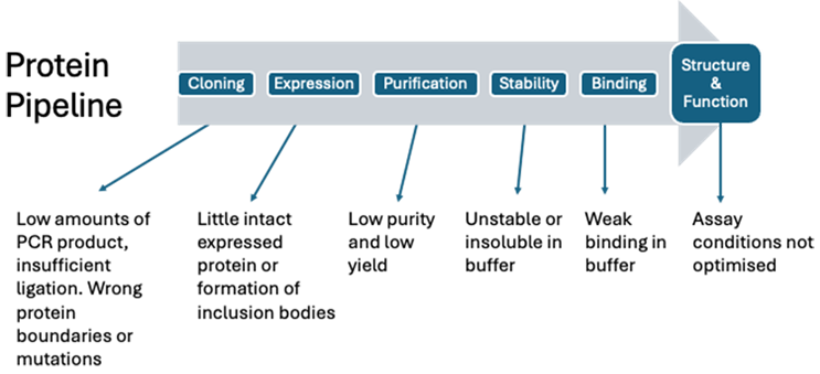
Figure 1: A typical protein production and characterization pipeline highlighting typical conditions that need optimizing.
At each stage, one can try to optimize factors by changing the levels of just one factor at a time (OFAT), although this is not very efficient and yields limited insight into your system. On the other hand, DoE is a statistical method used to set up several runs that change all factors simultaneously to help you explore how these different factors and their interactions influence a specific outcome, and it can quicky find the optimal factor levels to maximize yield.
In this article, we will focus on 2-level factorial designs, which illustrate the principles and power of the DoE approach and usually allow you to maximize 80% gain from just 20% of the effort. Other designs include unbalanced incomplete factorials for screening and response surface methods (RSM) for complete characterization/optimization.
Interestingly, 65% of delegates at PEGS24 reported not currently using DoE approaches and, of those who do, the majority most often use 2-level factorial designs.
The first step in generating a 2-level factorial design is to identify the factors that may be responsible for a given step in the protein pipeline. Three areas we commonly optimize are protein expression, purification, and stability (Figure 2).
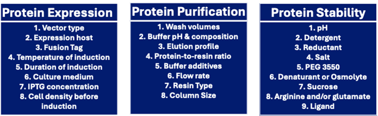
Figure 2: Possible factors affecting protein expression, purification, and stability.
Interestingly, for the delegates of PEGS24, most protein areas were explored with DoE (Figure 3).
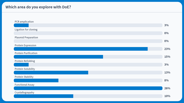
Figure 3: Survey of PEGS24 delegates on which area they explore with DoE; the most popular area was to optimize a functional assay.
We will briefly go through a typical example of protein expression in E.coli that has been explored more fully in a recently published article. Here we choose four factors that often affect protein expression and define two levels, a low level (-1) and a high level (+1), as can be seen in Figure 4.

Figure 4: An overview of the four factors and their chosen high and low levels to try to optimize protein expression.
Spreadsheet DoE is a series of five spreadsheets allowing you to explore systems affected by three to six factors in different numbers of runs using 2-level factorial designs. We use the C tab in the 4.8 spreadsheet (four factors in a minimum of eight runs), which I have provided on Zenodo. This sets up eight runs where the responses (amount of protein) to each experiment are entered by the researcher in the final green shaded column (Figure 5).
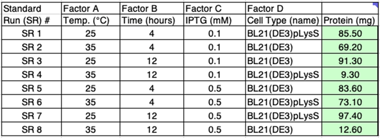
Figure 5: The eight runs designed by spreadsheet DoE to explore four factors at 2-levels. The runs are a fraction of the full factorial that would require 16 runs.
Spreadsheet DoE will help you check if the responses need transforming in any way; in this case, no transformation is required. Next, the effect of each factor/interaction and their sum of squared deviations (SS) are calculated using equations 1 and 2, respectively, and are included in a spreadsheet DoE table (Figure 6).
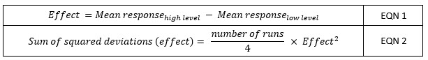
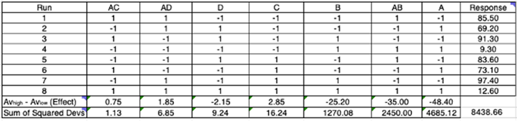
Figure 6: Each run has factors A, B, C, and D at either the high or low level. Interaction terms are also included in this table and their levels are determined by multiplying the component levels together. The factor/interaction terms are ordered from right to left based on the size of the effect (here, factor A has the biggest effect, calculated using EQN 1). The SS for each term (calculated using EQN 2) is also given and tells us how much the change in level of that term contributes to the total variability in the response (calculated by summing of all SS terms (8,438.66) or by simply calculating the SS of the responses).

Next, a half normal probability plot is made by spreadsheet DoE to estimate which terms to include in a regression model (Figure 7). In this case, the circled terms A, AB, and B lie off the line made by the earlier points and will likely help explain most of the variability of the response seen across the eight runs.
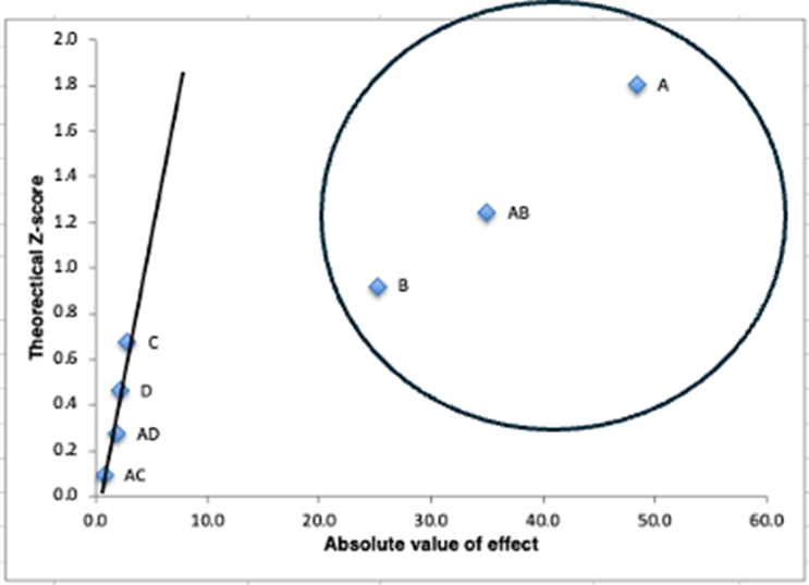
Figure 7: Spreadsheet DoE generates a half normal probability plot, where any terms that lie off the line (as indicated by the circle) are considered “signal” as opposed to “noise” and may be useful to include in the regression model.
Next, spreadsheet DoE will form a linear regression model (EQN 3). This is a predictive equation that attempts to predict the response based on the levels (-1 or +1) for factors A and B in this case.
Response (mg of protein) = 65.3 - 24*A - 17.5*AB – 12.6*B EQN 3
This equation is extremely useful as it allows us to say that factors A and B determine the response, while factors C and D make no significant impact (since they are missing from the equation). Furthermore, with a coefficient of 24, factor A has the biggest influence over the response. Interestingly, A and B also have an interaction, since there is a -17.5*AB term. This suggests that choosing a low level for A and a high level for B would maximize the response. Interaction terms are one of the most powerful insights that the DoE approach provides. An interaction shows that there is a synergy or anti-synergy between factors; in other words, the effect of changing levels for one factor depends on the level of the other factor.
This information can allow you to optimize a system more efficiently than the OFAT approach. We would therefore grow our E. coli cells containing our plasmid at 25 degrees C (low level for factor A) for 12 hours (high level for factor B) with either high or low levels for IPTG concentration (factor C) and either cell type (factor D).
Analysis of variance (ANOVA) is performed by spreadsheet DoE to determine a measure of confidence in the above model (Figure 8). Confidence is high for the model and its terms (significance >95%) as well as having good R-squared values. Spreadsheet DoE also summarizes ANOVA statistics for other models that include a different number of terms. Furthermore, it checks model assumptions by analyzing residuals in some diagnostic plots, which, in this example, give plots that validate these assumptions.
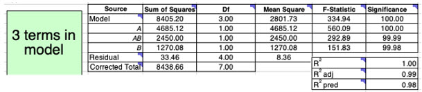
Figure 8: ANOVA table for a linear regression model that contains three terms: A, AB, and B. The mean square (variance) is calculated by dividing the SS by the degrees of freedom (df). The Fstatistic is the ratio of the variance of the term/s to the variance of the residual (noise); the higher the value, the more significant it is. Significance is given as a percentage, where >95% is deemed significant (equivalent to p-value < 0.05).
Although we have focussed on tab C (eight runs), there are four other designs investigating four factors that allow you to gain independent model error estimation, confidence in predicting outside of factor levels tested, and the ability to run experiments in separate blocks, i.e., half the runs one day and the other half another day (Figure 9). These can all be explored further in spreadsheet DoE.
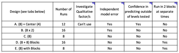
Figure 9: The design used in each spreadsheet (this example is for the 4.8 spreadsheet) will depend on what type of factor you wish to explore, how much error information and predictive power you wish to have, and whether you wish to run all experiments at the same time. In the example above we used the C tab, which requires eight runs to be tested.
The goal of spreadsheet DoE is to provide a simple tool for implementing 2-level factorials to the protein pipeline and beyond by demystifying the DoE approach. The spreadsheets are free to download and contain simple-to-follow instructions, simple spreadsheet formulae, and educational comments throughout to allow any researcher to start their own optimization.
I am also interested in receiving from the community any protein-related designs that have been completed to look for common trends and share these insights in a future study. DoE is a powerful approach that should be accessible to anyone, and you are encouraged to download and explore the spreadsheets so they can be applied to your system to help you save time and provide deeper insight into your system. Have fun using DoE!
Spreadsheets
The five spreadsheet DoE workbooks and the 4.8 spreadsheet with the example data used in this article are freely available to download and explore at this link.
About The Author:
 Elliott Stollar, Ph.D., is a senior lecturer and biochemistry program director at the University of Liverpool and an honorary member of the university’s Department of Biochemistry, Cell and Systems Biology. Previously, he worked at Eastern New Mexico University and at Mount Allison University in New Brunswick. He completed a post-doctoral fellowship at the Hospital for Sick Children and the University of Toronto. He received his Ph.D. from Cambridge University. Connect with him on LinkedIn.