Principles And Concepts Of System Risk Structures For Understanding & Managing Risks

Fundamentally, all risks are the same. Although assuring biopharmaceutical product quality, increasing the reliability of manufacturing processes, assuring worker safety, and minimizing personal health risks all look and feel different, a truly effective risk analysis method should provide insights to and understanding of the fundamental properties and attributes that underlie every type of risk. This article, the first of a series, describes how system risk structures (SRS) can be used to understand and manage both simple risk situations as well as complex risk landscapes quickly and efficiently. The second article in this series will apply SRS concepts to analyzing COVID-19 pandemic risks¹ and additional articles will describe other risk landscapes for managing CDMO risks, building contamination control strategies (CCS), providing safer work environments, and better managing projects.

Fundamental Concepts Underlying SRS

Risks are typically defined, viewed, analyzed, and managed as events. While this approach can effectively deal with a specific risk event, it provides little insight or understanding about how a portfolio of risk events should be managed in the context of the surrounding risk landscape.

SRS is based on three fundamental principles:

1. A risk is defined not as an event but as a possible threat event that enters a system that might control the threat’s ability to produce an output consequence event. All risks must be defined by a complete cause and effect relationship that identifies the threat event, a connecting system, and the resulting consequence event.
2. The only difference between a threat event and a consequence event is the system that produces it.
3. Threat events flow through sequences and networks of systems to produce a concerning final consequence event.

Contrary to common risk management practices of evaluating risks based on the impact and uncertainty of a single event, a risk must be evaluated based on the following three attributes that cover the entire cause–system–effect relationship:

• Severity – the impact, bad or good, of an event on one or more subjects or systems. A risk can be measured according to one or more severities. Severity can usually be objectively measured in terms of monetary loss (or gain) or physical impact or injury (or benefit). However, severity can also be subjectively measured in terms of perceived possible anguish (or joy) or pain and suffering (or pleasure). If the severity of the threat and consequence have the same units of measurement, then the system can either attenuate or accentuate the risk’s severity.
• Likelihood – Likelihood must be expressed as a probability between certain (one) and impossible (zero). For both threat and consequence events, the likelihood of occurrence is the probability the event will occur. For the connecting system, the likelihood of not controlling the threat is the probability that the system will fail to control the causal threat event producing the consequence event. Thus, the system can modify the threat’s likelihood of producing the consequence.
• Observer Uncertainty – Human perception has an impact on both severity and likelihood because of the risk observer’s or evaluator’s level of knowledge or ignorance, information or misinformation, experience or lack thereof, and personal priorities, biases, perceptions, and prejudices. The impact of observer uncertainty can range from being trivial for well-characterized simple risks to a dominant attribute for complex risks dependent on human judgements and interactions.

In a perfect world, the knowledge level would be complete and accurate for evaluating both severity and likelihood. But in the real world, the third attribute can have a significant impact on how both severity and likelihood are evaluated and managed.

In the case of building a reliable bioreactor, the first attribute, severity, is relatively simple, and the second attribute can be assessed by experts and verified by experimental methods. While the third attribute usually has minimal impact, in CCS development, it can have a significant impact. Considerable disagreement exists between industry experts and regulatory agencies on this.² While the experts, based on their considerable experience, feel that contamination risks can be sufficiently controlled with relatively straightforward sophisticated equipment, e.g., isolators, regulatory agencies take a much more conservative approach, as reflected in comprehensive and highly restrictive guidelines such as those in EUA’s Annex 1.³ On the other hand, COVID-19 risks provide an excellent example of how the third attribute sometimes plays a dominant role in the way many important healthcare risk decisions are made.¹

Given the high uncertainty and noisy information that surrounds and permeates almost all risks, determining a risk’s severity and likelihood of occurrence to the correct order of magnitude is usually sufficient for making good risk management and acceptance decisions. The challenge of any risk analysis approach is to evaluate and communicate the first two attributes such that the negative impact of the third attribute can be minimized.

System Risk Structures

SRS’s fundamental element shown in Figure 1 graphically describes the threat-system-consequence (TSC) definition of the first principle. The TSC definition covers both good and bad events.⁴

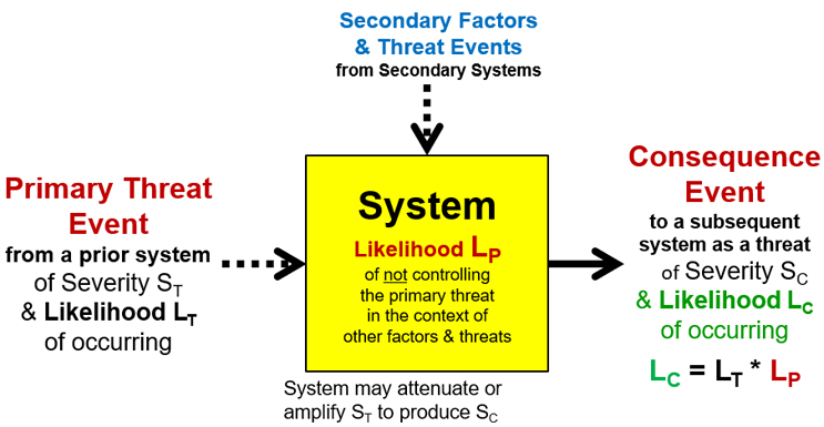
Figure 1 – A threat–system–consequence (TSC) definition of a risk: A possible threat (opportunity) of severity S_T and likelihood of occurring L_T passes through a system that has a likelihood of L_P of failing to control the threat, resulting in a risk (benefit) consequence of severity S_C and likelihood of L_C.^4,5 The likelihood L_C is equal to the product of L_T and L_P. The effectiveness of the system of controlling the primary threat is impacted by other input factors and threats. The system may also modify the severity of the threat’s S_T impact on the severity of the consequence S_C.

A system is defined as anything that takes an input and produces an output. People, equipment, procedures, processes, unit operations, etc. are viewed as systems. Systems vary widely in their ability to control threats. Some systems are very weak and highly unlikely to control the threat, while others can be very robust with a very high likelihood of controlling the threat. The system’s failure to control the threat L_P is impacted by secondary factors and other possible threat events. A subjective estimate of L_P is possible using thought experiments that evaluate the mechanism by which the system might allow the threat to produce the consequence.⁵ However, thought experiments are subject to considerable observer uncertainty based on the level of knowledge, experiences, and biases of the observer.⁵ In some cases, the system’s ability to detect or measure the threat is a critical part of controlling the threat.

In addition to the first three principles, SRS has the following additional principles:

4. All inputs to a system are possible threats, and all outputs are “at risk” and can be viewed as possible risk consequences.
5. Most risks can be effectively modeled as short linear sequences of one or more risk TLC elements.
6. A threat event can cause one or more consequence events described as different risks.
7. A consequence event can be caused by one or more threat events described as different risks.
8. Systems may be combined or subdivided as required to better understand, manage, and communicate the flow of threats.
9. Severities (S_T & S_C) and likelihoods (L_T, L_P, & L_C) can be initially estimated subjectively by an observer or SME team based on the available knowledge and experience but should be quantitatively re-estimated as appropriate using additional information, data, and statistical analysis whenever possible to minimize observer bias.
10. Very complex risks having significant secondary factors or more than one primary threat may require analysis using a probabilistic network of TLC elements. The use of TLC networks is not covered in this article.

A final SRS requirement is the question: “Is sufficient objective information and knowledge available, and have biases, prejudices, or misinformation been properly controlled?”

SRS’s third principle uses the basic element in Figure 1 to build sequences and networks to describe more complex risk landscapes. Figure 2 shows how systems can be linked together to structure the flow of threats through a sequence or network of systems.

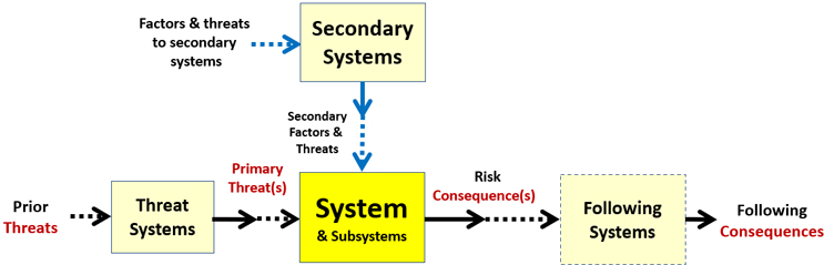
Figure 2 – Risk elements shown in Figure 1 can be connected to describe how threats flow through systems to produce consequences.

The TLC definition can be used to build relatively straightforward sequential risk landscapes. Complex landscapes can be qualitatively evaluated by identifying how multiple threats might flow through networks and be combined to result in a consequence of concern.

The real world is noisy, with many systems having many inputs and factors that could impact the performance of systems. That noise can make it difficult to precisely evaluate in quantitative terms a risk event’s severity and likelihood. However, most risks can be effectively managed by making order-of-magnitude estimates of both attributes. Converting very complex risk landscapes that look like mazes into straightforward approachable problems remains the ultimate challenge of analyzing many risks.

To assess a risk’s significance, its severity and likelihood of occurrence can be estimated and then rated using the following tables. Table 1 provides both objective and subjective ratings of a risk event’s severity by providing a rating value between 0 (no impact) to 7+ (catastrophic) based on an order-of-magnitude logarithmic value of the objective scale.

Table 1 – A risk event’s potential or actual impact severity can be evaluated on a logarithmic scale from 0, no impact, to 7+, catastrophic. The column on the left is a quantitative scale while the one on the right is a subjective scale for an observer quickly summarizing a risk event’s impact. A normal risk analysis would usually start subjectively and transition when appropriate to an objective evaluation as additional experience, knowledge, and data are gathered. In some cases, the system can attenuate or amplify S_T to produce S_C. A symmetrical scale for benefits is left to the reader.⁴

Table 1 is used to evaluate both the threat’s potential impact severity S_T and the consequence’s impact severity S_C. The most important severity is S_C, with the severity of the threat S_T being more of an estimated potential impact. Some threats are insignificant, while major threats can range from an inconsequential-looking trigger (e.g., a highly toxic poison) that enters and profoundly affects the system to produce significant consequences, to a major event that overwhelms the systems to produce major consequences (e.g., a 9+ magnitude earthquake). In both cases, the likelihood of the threat event L_T is the primary risk management consideration.

As shown in Figure 1, SRS likelihoods fall into two categories.  The first is a risk event’s (either the threat or the consequence) likelihood of occurrence as shown in Table 2.

Table 2 – Objective and subjective event likelihood of occurrence rating tables. On the left is an objective scale for the likelihood stated as a probability of a threat or consequence event. On the right is a subjective scale with likelihood rating in the middle column based on the log of the objective scale.

The other likelihood is the probability of a system controlling the threat as shown in Table 3.

Table 3 – Objective and subjective scales for rating the probability (likelihood) of a system failing to control a threat. The two scales produce a rating between 0 (no control) and ≤ -7 (barrier) based on the logarithm of the objective scale.

Because the SRS includes a system connecting the threat event and the consequence event, the system’s likelihood of not controlling the threat is a central element to understanding a risk. As described previously, the likelihood of a system controlling a threat covers the entire scale from L_P^ = 0 (no control) to L_P^ ≤ -7 (a barrier).

Once the TLC element has been identified, the likelihood tables can be used to rate the likelihood of occurrence of both the threat and consequence events as well as the likelihood of the connecting system propagating the threat. A risk analysis is initiated with a subjective estimate of the risk consequence’s likelihood L_C^ shown in Table 2, followed by estimating how likely the threat is to occur L_T^ and then estimating how likely the system is to control the threat L_P^. The consequence’s likelihood can then be reevaluated by adding L_T^ and L_P^ together. If the initial L_C^ differs significantly from the second, the analysis should gather additional information to improve the estimates.

While the severity and likelihood ratings provide a simple and convenient measure, they can lead to some confusion. Severity is simple, as shown in Table 1, with the numerical rating from 0 to 7+ being the exponent of the objective severity rating. But likelihood ratings can be confusing because the probability rating L_C or L_P = 1 (certain) results in a numerical rating L_C^ or L_P^ = 0, while the probability rating of L_C or L_P = 0 (impossible) results in an undefined L_C^ or L_P^ because the logarithm of zero is an undefined value, as shown in Tables 2 and 3.

Perhaps the most difficult challenge of evaluating any risk is estimating the likelihood of occurrence of the risk events. If frequency data is available, it should be used in estimating an event’s likelihood. For measuring the performance of systems, performance data is extremely valuable in estimating L_P^. In the absence of data or to supplement available information, an alternative method is to use thought experiments based on an understanding of the system’s mechanism by which the threat event passes through the system’s possible control mechanisms to result in the consequence event. Prospective Causal Risk Modelling (PCRM) is one method that can be used to subjectively estimate the likelihood of both risk events L_T and L_C, as well as the system’s performance L_P.⁵

After S_C^ and L_C^ are estimated, a quick assessment of the risk’s likely impact can be achieved by adding the two attributes S_C^ and L_C^ together to provide an adjusted risk likelihood (ARL). Visually, the ARL describes the risk as shown in Figure 3.

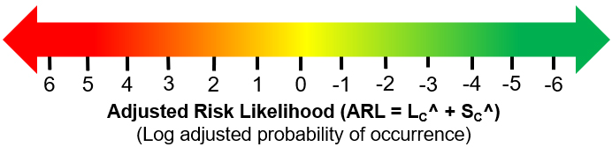
Figure 3 – The ARL provides a quick method of valuing a risk. The ARL is calculated by adding the severity and likelihood ratings together. Generally, the lower the ARL, the better.⁶

For a better conceptual understanding, the ARL can also be viewed as an adjusted risk severity (ARS) where the severity is adjusted by the likelihood of occurrence. The net severity of a risk is reduced when the risk becomes less likely to occur.⁶

Positive ARL values usually suggest taking a harder look at controlling the risk by improving the L_Ps of one or more systems or even adding new systems to improve control, while negative ARLs suggest the risk’s overall impact may not require additional remediation.

An interesting property of the ARL is that some risks have similar ARL values over a range of severities.  For example, earthquakes with increasing severity are often counterbalanced by a decreasing likelihood of occurrence. Thus, the ARL for earthquakes would be based almost entirely on the seismic frequency history of a location. When comparing risks, the ARLs can be compared with the lower ARL likely being the lower risk. A similar approach can be used for assessing risk-benefit options.⁴

What is the difference between FMEA’s RPN and SRS’s ARL?⁶ The biggest difference is the RPN is calculated early in the analysis, while the SRS uses the ARL at the end of the analysis. Compressing two fundamentally different attributes into a single value will always result in a significant loss of information. The later the information is lost, the better. Since risks are usually identified by severity and managed by likelihood, preserving both attributes to the end of the analysis is vital for success.⁶

When using Tables 1, 2, and 3, the impact of observer uncertainty – a risk’s third attribute – should always be carefully considered. Any values selected using the subjective criteria may or may not reflect a correct value when compared to many data points that objectively measure both an event’s severity in Table 1 and likelihood of occurrence in Table 2. Estimating how likely a system manages threats, as shown in Table 3, can be especially vulnerable to observer bias.

Summary And Future Work

SRS provides a simple view of how threat events become consequence events of concern. The approach can be used intuitively by individuals to provide a quick and efficient mechanism for viewing risks or by a team of experts to analyze complex risks. The method can start by initially looking at any of the three components — consequences, threats, or systems — to build an understanding of how threats might flow through a system to produce a consequence (good or bad) of concern.

SRS is a synthesis of many existing risk analysis methods. While its foundation is causal networks, it also shares commonly used risk analysis concepts imbedded in FMEA, FTA, HACCP, Bow-Tie, etc. Each method was simplified to its most basic principles and then combined to provide only the complexity necessary to describe a risk’s most fundamental attributes.

Much work remains to further develop and communicate SRS. Simple, conceptual methods that minimize mathematical complexity of building and analyzing TLC-based directed acyclic graph (DAG) networks to better describe causal relationships remain to be developed.⁷ By applying and demonstrating SRS and PCRM methods to both simple risks and complex risk landscapes, more usable methods for analyzing and communicating risks can be developed. Future articles in this series should aid in further understanding SRS and PCRM as a method of identifying, analyzing, evaluating, and managing risks.

References

1. Witcher, M. Using System Risk Structures To Evaluate COVID-19 Pandemic Risks, BioProcess Online, December 15, 2021. Upcoming.
2. Akers, J., J. Agalloco, & R. Madsen, Slow-walking The Isolator – A Cautionary Tale, BioProcess Online, Dec. 2, 2020. Slow-walking The Isolator — A Cautionary Tale (bioprocessonline.com)
3. EU GMP Annex 1: Manufacture of Sterile Medicinal Products – revision November 2008. https://www.gmp-compliance.org/files/guidemgr/annex%2001[2008].pdf
4. Witcher, M., Using System Risk Structure to Understand and Balance Risk/Benefit Trade-offs, BioProcess Online, April 23, 2021. Using System Risk Structures To Understand And Balance Risk Benefit Trade-offs (bioprocessonline.com)
5. Witcher MF. Estimating the uncertainty of structured pharmaceutical development and manufacturing process execution risks using a prospective causal risk model (PCRM). BioProcess J, 2019; 18.   https://doi.org/10.12665/J18OA.Witcher
6. Witcher, M., Rating Risk Events: Why We Should Replace The Risk Priority Number (RPN With The Adjusted Risk Likelihood (ARL), BioProcess Online, April 7, 2021 Rating Risk Events Why We Should Replace The Risk Priority Number (RPN) With The Adjusted Risk Likelihood (ARL) (bioprocessonline.com)
7. Sucar, L., Probabilistic Graphical Models – Principles and Applications, Springer, 2015.

About the Author

Mark F. Witcher, Ph.D., has over 35 years of experience in biopharmaceuticals. He currently consults with a few select companies. Previously, he worked for several engineering companies on feasibility and conceptual design studies for advanced biopharmaceutical manufacturing facilities. Witcher was an independent consultant in the biopharmaceutical industry for 15 years on operational issues related to: product and process development, strategic business development, clinical and commercial manufacturing, tech transfer, and facility design. He also taught courses on process validation for ISPE. He was previously the SVP of manufacturing operations for Covance Biotechnology Services, where he was responsible for the design, construction, start-up, and operation of their $50-million contract manufacturing facility. Prior to joining Covance, Witcher was VP of manufacturing at Amgen. You can reach him at witchermf@aol.com or on LinkedIn (linkedin.com/in/mark-witcher).