An Introduction To Sampling Plans

Sampling plans are used extensively throughout organizations regulated by the FDA. Most organizations have a statistical procedure that specifies a certain acceptable quality level (AQL) based on risk. (If not, they should!) However, most individuals just follow the requirements of the procedure without fully comprehending how sampling plans actually work.

Probability sampling is based on the fact that every member of a population has an equal chance of being selected. Basically, statistical sampling plans are used to make decisions on whether to accept or reject products. Statistical sampling plans are a commonly used quality control technique for incoming, in-process, and final inspection.

Sampling plans are used when testing is destructive and all parts would be consumed during testing, leaving no parts for commercial use or distribution, the cost of 100 percent inspection is very high, or 100 percent inspection takes too long.

Sampling plans are a means of identifying, not preventing, poor quality. Sampling plans are not a substitute for process control.

Sampling plans can be used for both variable and attribute data. Recall that variable data can be measured on a continuous scale and attribute data measures discrete data points, such as pass/fail, go/no-go, and things that can be counted.

All Sampling Is Subject To Risk

All statistical sampling is subject to risk. The risks are defined by the margin of error and confidence intervals. Ideally, a sampling plan should reject all “bad” lots while accepting all “good” lots. However, because sampling plans base decisions on a sample of the lot and not the entire lot, there is always a chance of making an incorrect decision. These errors are referred to as Producer’s Risk and Consumer’s Risk. Type I Alpha Error (α) Producer’s Risk is the probability of rejecting a good lot. Type II Beta Error (β) Consumer’s Risk is the probability of accepting a bad lot.

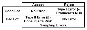
Figure 1: Producer’s and consumer’s risk

How Sampling Plans Work

All sampling plans utilize the concept of a lot (N), sample (n) drawn randomly from the lot, and an acceptance number (c). A lot is a whole — every member of a group — and a sample is a subset of a lot. For each lot inspected, we make an accept/reject decision with the accepted lots released to stock and the rejected lots segregated, labeled, and quarantined.

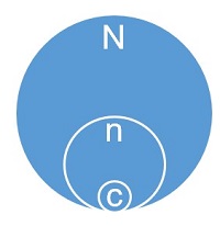
Figure 2: Graphical representation of a lot (N), sample (n), and acceptance number (c)

For example, a lot containing 2,500 (N) pieces is inspected using an AQL of 1.0, which requires 42 (n) pieces to be randomly selected from the lot and inspected. In this example, the acceptance number is 0 (c). If all 42 randomly selected pieces are inspected and all of the pieces meet the inspection criteria (zero failures), the lot is accepted (passes). However, if there is one failure, the lot is rejected (fails) and should be segregated, labeled, and quarantined until addressed by the Material Review Board (MRB).

Operating Characteristic Curve

The behavior of a sampling plan is described graphically by the sampling plan’s operating characteristic curve (OCC). Operating characteristic curves are generated using the binomial distribution or Poisson distribution, with the exception of C=0 sampling plans. The hypergeometric distribution is used to generate the operating characteristic curve for C=0 sampling plans. The curves can be easily constructed using reference tables, calculators, or spreadsheets.

The operating characteristic curve shows the probability of accepting lots of different quality levels for a specific sampling plan and helps discriminate between good and bad lots. The exact shape and location of the curve is defined by the sample size (n) and acceptance number (c) for the sampling plan.

The acceptable quality level (AQL) is a measure of the level of quality routinely accepted by that sampling plan. It is defined as the percent defective that the sampling plan will accept 95 percent of the time. This means lots at or better than the AQL are accepted at least 95 percent of the time and rejected at most 5 percent of the time. The AQL can be determined using the OCC by finding that quality level on the bottom axis that corresponds to a probability of acceptance of 0.95 (95 percent) on the left axis (see Figure 3).

The lot tolerance percent defective (LTPD) is the level of quality routinely rejected by the sampling plan. It is generally defined as the percent defective that the sampling plan will reject 90 percent of the time. In other words, this is also the percent defective that will be accepted by the sampling plan at most 10 percent of the time. This means that lots at or worse than the LTPD are rejected at least 90 percent of the time and accepted at most 10 percent of the time. The LTPD can be determined using the OCC by finding that quality level on the bottom axis that corresponds to a probability of acceptance of 0.10 (10 percent) on the left axis (see Figure 3).

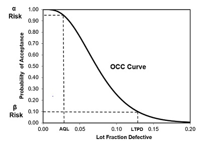
Figure 3: Example operating characteristic curve (OCC)

The acceptance number (c) has a significant impact on the shape of the OCC. As shown in Figure 4, as the acceptance number (c) increases, the producer’s risk (α) decreases and, inversely, as the acceptance number (c) decreases, the producer’s risk (α) increases. Additionally, as the acceptance number (c) increases, the consumer’s risk (β) increases and, inversely, as the acceptance number (c) decreases, the consumer’s risk (β) decreases. C=0 sampling plans developed by Nicholas Squeglia are widely accepted in the FDA regulated industries as they provide greater protection for the consumer.

Figure 4: Example pperating characteristic curve (OCC) for C=0, C=3, and C=5

An ideal/perfect OCC will yield no Type I Error (α) Producer’s Risk or Type II Error (β) Consumer’s Risk for a given lot fraction defective or less.

The OCC shown in Figure 5 is considered ideal/perfect. For this curve, a lot fraction defective of £ 0.25 will be accepted 100 percent of the time. In reality, the ideal/perfect OCC does not exist.

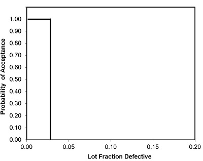
Figure 5: Theoretical perfect operating characteristic curve (OCC)

Conclusion

Sampling plans should be linked to risk. It should be obvious that more inspection is required and should be performed for higher-risk items and less sampling should be required and performed for lower-risk items. Ensure your training program provides some background on how and why sampling plans work for those performing sampling activities.

It’s worth repeating: Sampling plans are a means of identifying, not preventing, poor quality. Sampling plans are not a substitute for process control. An effective sampling program can be used to augment and support process control.

References:

1. ANSI/ASQ Z1.4-2008: Sampling Procedures and Tables for Inspection by Attributes
2. ANSI/ASQ Z1.9-2003 (R2013) Sampling Procedures and Tables for Inspection by Variables for Percent Nonconforming
3. Durivage, M.A., 2014, Practical Engineering, Process, and Reliability Statistics, Milwaukee, ASQ Quality Press
4. Squeglia, Nicholas K. 2008, Zero Acceptance Number Sampling Plans. 5th ed. Milwaukee: ASQ Quality Press.

About The Author:

Mark Allen Durivage has worked as a practitioner, educator, consultant, and author. He is managing principal consultant at Quality Systems Compliance LLC, an ASQ Fellow, and an SRE Fellow. He earned a BAS in computer aided machining from Siena Heights University and an MS in quality management from Eastern Michigan University. He holds several certifications, including CRE, CQE, CQA, CSQP, CSSBB, RAC (Global), and CTBS. He has written several books available through ASQ Quality Press, published articles in Quality Progress, and is a frequent contributor to Life Science Connect. Durivage resides in Lambertville, Michigan. Please feel free to email him at mark.durivage@qscompliance.com or connect with him on LinkedIn.